Chapter 4 A deeper understanding of Options
This chapter aims at digging a bit more into European options and the model used to price them: the Black-Scholes model.
I have asked myself a lot of questions about the following chapters, trying to figure out where to start and how deep into mathematics should I go?
My goal is to get you to have the best understanding of options as possible. Mathematics is not always useful and necessary as you can get a great sense of options with a good intuition. I mainly rely on intuition when teaching this material.
As it might help the more quantitative profiles among the readers to dig into the mathematics behind the Black-Scholes model, I decided to share the derivation of the Black-Scholes Equation in Appendix of this chapter. For the others, there is surely enough maths in this chapter anyway.
4.1 The Black-Scholes model
Black and Scholes developed a closed-form pricing formula for European options. The market assumptions behind their model are quite strong and contained:
- Constant volatility
- Constant interest rates
- Log-normality distributed stock prices
- Constant dividend yield
The concept of risk-neutral pricing is at the heart of the Black-Scholes model.
4.1.1 Risk-Neutral Pricing
In finance, when pricing an asset, a common technique is to discount the expected cashflows. The expected cashflows are calculated using the real-world probability of each cashflow and the risk adjustment takes the form of a higher discount rate.
In the theory of risk-neutral pricing, the real-world probabilities assigned to future cash flows are irrelevant, and we must obtain what are known as risk-neutral probabilities.
The fundamental assumption behind risk-neutral valuation is to use a replicating portfolio of assets with known prices to remove any risk. By the no-arbitrage condition, we can create a pricing model by setting the temporary risk-less hedged portfolio return to the risk-free rate instead of unknown market expectations. The amounts of assets needed to hedge determine the risk-neutral probabilities.
Under the aforementioned assumptions, the Black–Scholes theory considers options to be redundant in the sense that one can replicate the payoff of a European option on a stock using the stock itself and risk-free bonds.
As such, the key feature of the Black–Scholes framework is that it is preference-free: since options can be replicated, their theoretical values do not depend upon investors’ risk preferences, only upon the current stock price and its dynamics.
Therefore, an option can be valued as though the return on the underlying is riskless. This risk-neutral assumption behind the Black–Scholes model constitutes a great advantage in a trading environment. In the risk-neutral world, all cashflows can be discounted using the risk-free rate (r) whereas, in a real word, the discount rate should take into account the risk premium, which is more delicate.
A small example
Let me share with you a nice practical example that might help you to grasp the concept of risk-neutral valuation.
Suppose a first horse has 20% chance to win while a second horse has 80% chance to win.
\(10.000€\) is bet on the first horse and \(50.000€\) is bet on the second.
If odds are set to 4:1, then:
- The bookmaker may gain \(10.000€\) if the first horse wins \((50.000€ - 4*10.000€)\).
- The bookmaker may loose \(2500€\) if the second horse wins \((10.000€ - 1/4*50.000€)\).
- The bookmaker’s expected profit is 0 \((0.2*10.000€ + 0.8*-2500€)\).
If odds are now set to 5:1, then the bookmaker won’t lose or gain money no matter which horse wins. That represents the risk-neutral probabilities.
4.2 European Call Options
4.2.1 Introduction
A call option is a financial contract that gives its holder the right, but not the obligation, to buy a specified amount (nominal = N) of an underlying asset (S) at a specified price (strike price = K) within a specific time period (maturity = T).
Therefore, a call buyer profits when the underlying asset increases in price.
It is important to distinguish between payoff at maturity, premium or market price and profit.
4.2.2 Buyer’s payoff at maturity
\(\boxed{C_T = Max(S_T \; - \; K, 0) = (S_T \; - \; K)^+ = \; 1_{\{ S_T > K \}} (S_T \; - \; K) }\)
It is good that you get familiar with these notations as soon as possible as you will see them a lot through this material. You must know them perfectly when working in equity derivatives.
\(1_{S_T>K}\) is an indicator function having a value of 1 if \(S_T\) > K and 0 otherwise.
Let’s plot the Call payoff with respect to the underlying spot price.

Fig: 4.1 : Call Payoff at Maturity
As you can see in the graph, the option’s strike price is the key point which divides the payoff function in two parts. Below the strike, the payoff chart is constant and null.
Above the strike the line is upward sloping, as the call option’s payoff is rising in proportion with the underlying price.
So you have got nothing to lose at maturity when buying a call option. you will therefore have to pay for this right!
How much?
Well, that’s given by the call option premium and we will see now how to calculate it.
The good thing when buying a call option is that your loss is always limited to the premium paid for being long the call option. Inversely, when selling a call option, your potential loss is illimited.
The good thing with a long call trade is that your loss is always limited to the initial cost.
4.3 European Put Options
4.3.1 Introduction
A put option is a financial contract that give its holder the right, but not the obligation, to sell a specified amount (nominal = N) of an underlying asset (= S) at a specified price (strike price = K) within a specific time period (maturity = T).
Therefore, a put buyer profits when the underlying asset decreases in price.
It is important to distinguish between payoff at maturity, premium or market price and profit.
4.3.2 Buyer’s payoff at maturity
\(\boxed{P_T = Max(K \; - \; S_T, 0) = (K \; - \; S_T)^+ = \; 1_{\{ S_T < K \}} (K \; - \; S_T) }\)
Let’s plot the Put payoff with respect to the underlying spot price.

Fig: 4.4 : Put Payoff at Maturity
As you can see in the graph, the option’s strike price is the key point which divides the payoff function in two parts. Below the strike, the payoff chart is in the positive territory and the payoff increases as the underlying price goes down. This relationship is linear.
Above the strike, the payoff is constant and null.
So you have got nothing to lose at maturity when buying a put option. you will therefore have to pay for this right!
How much?
Well, that’s given by the put option premium and we will see now how to calculate it.
The good thing when buying a put option is that your loss is always limited to the premium paid for being long the put option. Inversely, when selling a put option, your potential loss can be quite substantial if the underlying stock price plunges.
4.4 Intrinsic Value and Time Value
4.4.1 Introduction
The concept of time value is very simple and intricate at the same time.
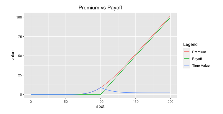
The time value can be defined as the value of the option above the intrinsic value. You should know by now that the intrinsic value is the value any given option would have if it were exercised today.
You can always express an option price as the sum of its intrinsic value and its time value.
\(\boxed{Option \; Price = Intrinsic \; Value + Time \; Value}\)
Call Intrinsic Value = Max(0; S - K)
Put Intrinsic Value = Max(0; K – S)
At first sight, one might assume that time value has to be a positive number. Well, if we take out-of-the money options, their intrinsic values are zero but their prices are typically not zero. Therefore, this differential is positive. Hence, we intuitively expect the time value to be positive.
While it is most often positive, we have seen that it could also be negative in some situations.
We will now discuss the attitude of time on call and put options.
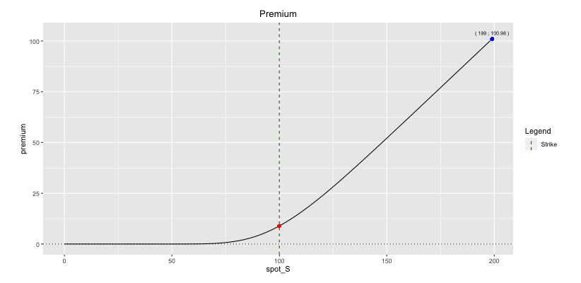
4.4.2 Time Value of Call Options
Let us prove the positive attitude of the time on a call option by considering both OTM and ITM cases.
4.4.2.1 OTM and ATM Cases
OTM and ATM cases are trivial since premium is always positive and hence always more than the intrinsic value being worthless.
4.4.2.2 ITM Case
Suppose we own an in-the-money European call and want to lock the intrinsic value \(S_0 - K\). We can do it by selling forward the stock to freeze the price risk.
If the option ends up in-the-money, we will exercise the option and our cashflow will be: \(\boxed{S_0e^{(r \; - \; q)T} \; - \; K}\)
If the option ends up out-of-the-money, we won’t exercise it and the only cashflow will be: \(\boxed{S_0e^{(r \; - \; q) T} \; - S_T > S_0 e^{(r \; - \; q)T} \; - K}\)
If \(S_0e^{(r \; - \; q)T} \; - K\) is always bigger than the intrinsic value \(S_0 - K\), then the cost of this hedge (= the call price) needs to be above this final guaranteed outcome (by the no-arbitrage argument) \(\Rightarrow\) \(\boxed{Call \; price > S_0-K}\). In such cases, the time value will always be positive.
On the contrary, if this inequality is not always verified, time value can happen to be negative.
4.4.2.3 Conclusion
The time value of a Call option is always positive except for deep ITM calls when (r - q) is negative. This is the case when the dividend yield of the underlying stock is higher than the risk-free interest rate (q > r). Note that this includes the case of a non-dividend paying stock in a negative interest-rate world.
The always positive time value of Call options on non-dividend paying stocks in a positive rates environment explains why there is no difference in premium between American and European Calls on such underlyings.
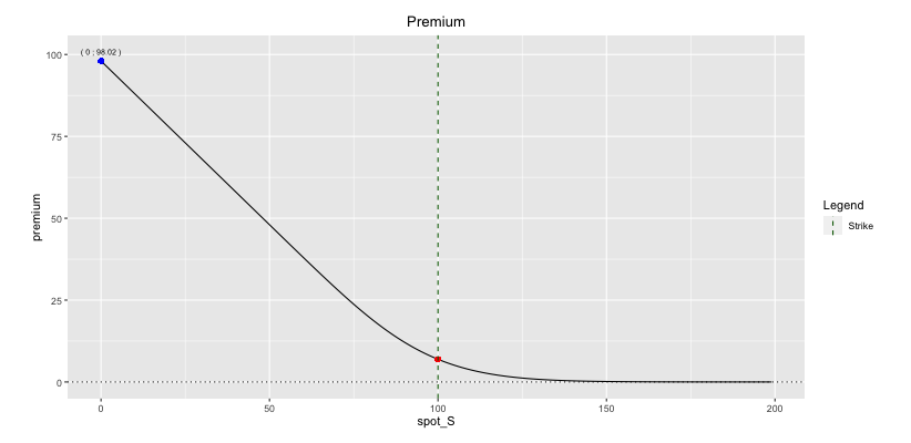
4.4.3 Time Value of Put Options
We can wonder why this argument does not hold for put options. It looks reasonable to do the same thing.
4.4.3.1 OTM and ATM Cases
OTM and ATM cases are trivial since premium is always positive and hence always more than the intrinsic value being worthless.
4.4.3.2 ITM Case
For hedging in-the-money put options, we need to buy forward the stock to freeze the price risk and lock the intrinsic value \(K - S_0\).
If option ends up ITM, we will exercise the option and our cashflow will be: \(\boxed{K \; - \; S_0e^{(r \; - \; q) T}}\)
If option ends OTM, we won’t exercise and our cashflow will be: \(\boxed{S_T \; - \; S_0 e^{(r \; - \; q) T} \; > \; K \; - \; S_0 e^{(r \; - \; q) T}}\)
By the no-arbitrage argument, the cost of this hedge needs to be above this final guaranteed outcome. \(\Rightarrow\) \(\boxed{Put \; price > K-S_0 \; e^{(r \; - \; q)T}}\)
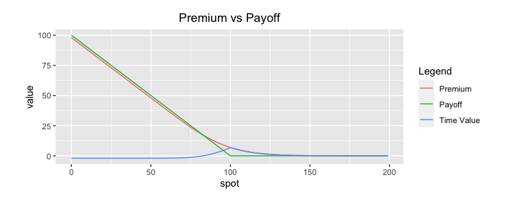
However, since \(\boxed{ K \; - \; S_0 e^{(r \; - \; q)T} \; < \; K - S_0}\) when interest rate is bigger than the dividend yield of the underlying stock, it becomes possible that the premium is less than the intrinsic value and therefore the time value negative.
4.4.3.3 Conclusion
The time value of a Put option is always positive except for deep ITM Puts when the interest rate is bigger than the dividend yield (r > q). This happens more frequently as some stocks do not pay dividends. That was the case in Fig: 3.6 where I plot a 1-year put option on a non-dividend paying stock in a 2% interest-rate world.
So the situations where the time value is negative can be traced back to the cashflows. Receiving money now or receiving the same amount of money in the future is not the same. And the direction of the cashflows in case of the put option are reversed!
The whole construction here is a nice example of proxy hedging the option.
However, the outcome of the hedging strategy is unsure. We had inequalities rather than equalities.
The reason for the residual risk has to do with the fundamental aspect of options.
We started by saying that the option was ITM and hedging accordingly. If then, afterwards, it turns out to be OTM, there arises a risk/uncertainty in the value the hedge will produce. The balance between the option and the hedge is broken at that time.
4.5 The Cost of Hedging
I will never emphasize it enough but it is very important to remember that the price of an option should reflect the cost of hedging it!
There are many parameters to consider when pricing an option: interest rates, volatility, repo, dividends, exchange rate, correlation, etc.
For european options, these parameters can be inserted into the Black-Scholes formula to get their prices. Such closed-form solutions that reflect the cost of hedging do not always exist for more sophisticated payoffs. Moving towards more complicated options, it is essential that you keep in mind that the cost of an option should reflect the cost of hedging the risks entailed!
Often all the risks are not hedgeable so that the product won’t be fully hedged to replication. It will then be hedged so that the remaining risk exposures are tolerable according to the risk department.
Pricing an exotic product therefore comes down to understand, manage and price the underlying risks.
4.6 The Call-Put Parity
4.6.1 Introduction
Put–call parity specifies a relationship between the prices of european call and put options with the identical strike price K and expiry T. Perhaps the most important feature of put–call parity is that it must be satisfied at all times, in a model independent manner. A violation of this leads to arbitrage opportunities.
4.6.2 The Call-Put relationship
\(\boxed{Call(K,T) - Put(K,T) =S_0e^{-qT} - Ke^{-rT}}\)
The left side of this equality consists of a portfolio A, which is a long call position and a short position with the same strike price and maturity (K,T) on the same underlying asset S.
The right side of this equality consists of a portfolio B, which is a long position in a forward contract that gives its holder the obligation to buy the underlying asset A at a price K at maturity T. In all states, both portfolio A and B have the same payoff at maturity.
As early exercise is not possible for European options, if the values of these two portfolios are the same at the expiry of the options, then the present values of these portfolios must also be the same. If it is not the case, an investor can arbitrage and make a risk-free profit by purchasing the less expensive portfolio, selling the more expensive one and holding the long-short position to maturity.
Accordingly, we have the following price equalities:
\(\boxed{Call(K,T) - Put(K,T) = Forward(K,T)}\)
and
\(\boxed{Forward(K,T) = S_0e^{-qT} - Ke^{-rT}}\)

Fig: 4.7 : Call-Put Parity: Call - Put = Synthetic Forward


 Descending curve: long put ⇒ negative delta ⇒ short forward.